There are currently three major types of mathematical techniques used in the Hobby School visualization tools to forecast future trends and detect historic patterns in data sets.  These three techniques are interpolating polynomial spline fitting, approximating least squares polynomial curve fitting, and discrete sample spectral analysis.  Each of these three approaches offer benefits when applied individually.  Additionally, any or all can be used concurrently to glean even more insight and information.

Interpolating polynomial spline fitting

The first use of interpolating polynomial spline fitting appeared in the University of Houston population study visualization "PopuView".  In the tool, a cubic polynomial is used to interpolate over 270 zip-code based census variables from four known sample points. The sample points included: The 1990 census, the 2000 census, the 2007 census update, and the 2012 census forecast.

Interpolating polynomial spline fitting was chosen due to its ability to determine a representative equation that has three desirable properties when only a small number of samples are available: precise interpolation of known sample points, C1 continuity (differentiable) between sample points, and estimation of functional behavior beyond the last sample point. For example, the first property guarantees recovery of exact year 2000 census values from the equation if the user sets the time parameter to the year 2000.

The specific polynomial used is similar to the Catmull-Rom cubic spline.  The primary difference is due to the non-uniform spacing of the census data samples over time (1990, 2000, 2007, & 2012). As a result, the construction of the cubic polynomial is accomplished via the linear blending of two Lagrange parabolas calculated with the appropriate time parameter separation. Figure 1 depicts the construction of the cubic polynomial.  

Figure  1 - blended Lagrange parabolas with non-uniform parameter spacing

Approximating least squares polynomial curve fitting

The first use of approximating least squares polynomial curve fitting appeared in the Department of Family and Protective Services (DFPS) capacity study visualization tool. The tool, called "DFPSView", is capable of generating forecasts interactively from a database of monthly child placements containing over 1.8 million records.  The number of variables in the DFPS database allow for over a million forecast permutations.

Approximating least squares polynomial curve fitting calculates a representative equation that evaluates, as closely as possible (in a least-squares sense), to the input sample points.  It was selected for three specific reasons: support for a large number of samples, direct calculation of the approximation error for known samples, and multiple degree estimation of the representative equation. For example, the last reason allows a set of equations (linear, quadratic, cubic, etc.) to be determined and tested for consistency on a general trend -- increasing, decreasing, etc.

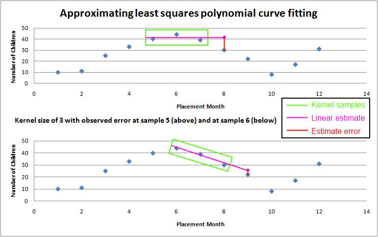
The specific method for least-squares estimation is similar to polynomial regression.  The major difference is that, before coefficients are determined, a variable sized sample kernel (2 ≤ size ≤ total samples) is passed over each sample in the input data set. Samples in the kernel are used to estimate their nearest neighbor and the differences between the estimates and actual samples are accumulated.  The kernel size that yields the lowest error estimating the known sample points is then used to generate the polynomial that estimates the unknown samples.

This technique allows the software to impart local control (avoiding potential global artifacts) as not every sample point need be used to construct the representative polynomial. In many cases, a smaller set of samples yields a lower aggregate error when estimating known data points. Figure 2 depicts the sliding kernel approach used to estimate the best sample size for determining the representative polynomial.  

Figure 2 - variable kernel applied on a data subset to estimate error from known samples

Discrete sample spectral analysis

The first use of discrete sample spectral analysis occurred during the Greater Houston Partnership (GHP) Energy Task Force study.  In support of the study, a tool named "ClusterView" was created to examine seven different house-related metrics (7 degrees of freedom) which could all be represented on screen simultaneously.  Spectral analysis was primarily needed to determine the underlying reason the age of a house did not correlate strongly with the amount of energy it consumed.

Discrete sample spectral analysis calculates frequencies and phases shifts for sinusoids that can be summed together to estimate a function used to generate the input samples.  It was selected for three specific reasons: the estimated function interpolates the original samples precisely, noise reduction and filtering of data samples can be applied in the frequency domain, and current implementations evaluate in near-real time on modern computer hardware.  The second reason, for example, allows for a less "noisy" (but still representative) data set to be used in conjunction with the two trend analysis methods described above.

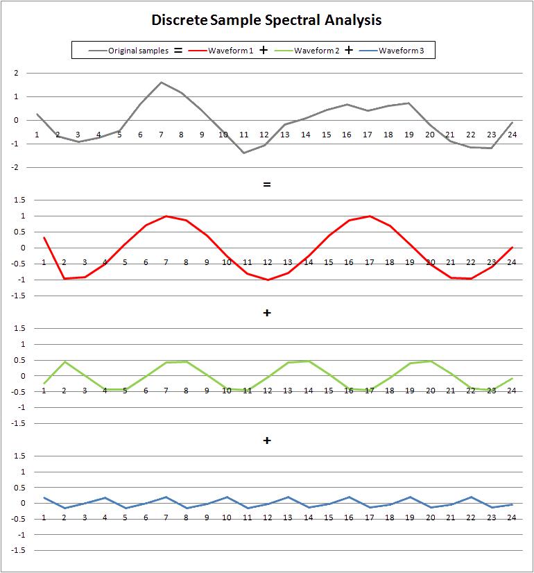
The technique used for spectral analysis is similar to the Fourier transform.  The primary difference is due to the fact that careful scaling and conversion of units must be performed to translate the results of analysis into useable and comprehensible information. Frequencies and shifts need to represent application dependent time intervals (cycles per month, periods per year, etc.) instead of their less appropriate signal/sampling theory counterparts (Hz, radians per second, etc.) Figure 3, below, demonstrates how three waveforms determined by discrete sample spectral analysis can be used to reconstruct an original sample data set.

Figure 3 - three waveforms that reconstruct an original input data set